WP1 — NEAR-FAULT SIMULATION CONSIDERING FAULT MECHANICS

Coordination: Hideo Aochi (BRGM)

Main partners: BRGM, Shimizu Corp., UGE, ENS, ARM, LMU

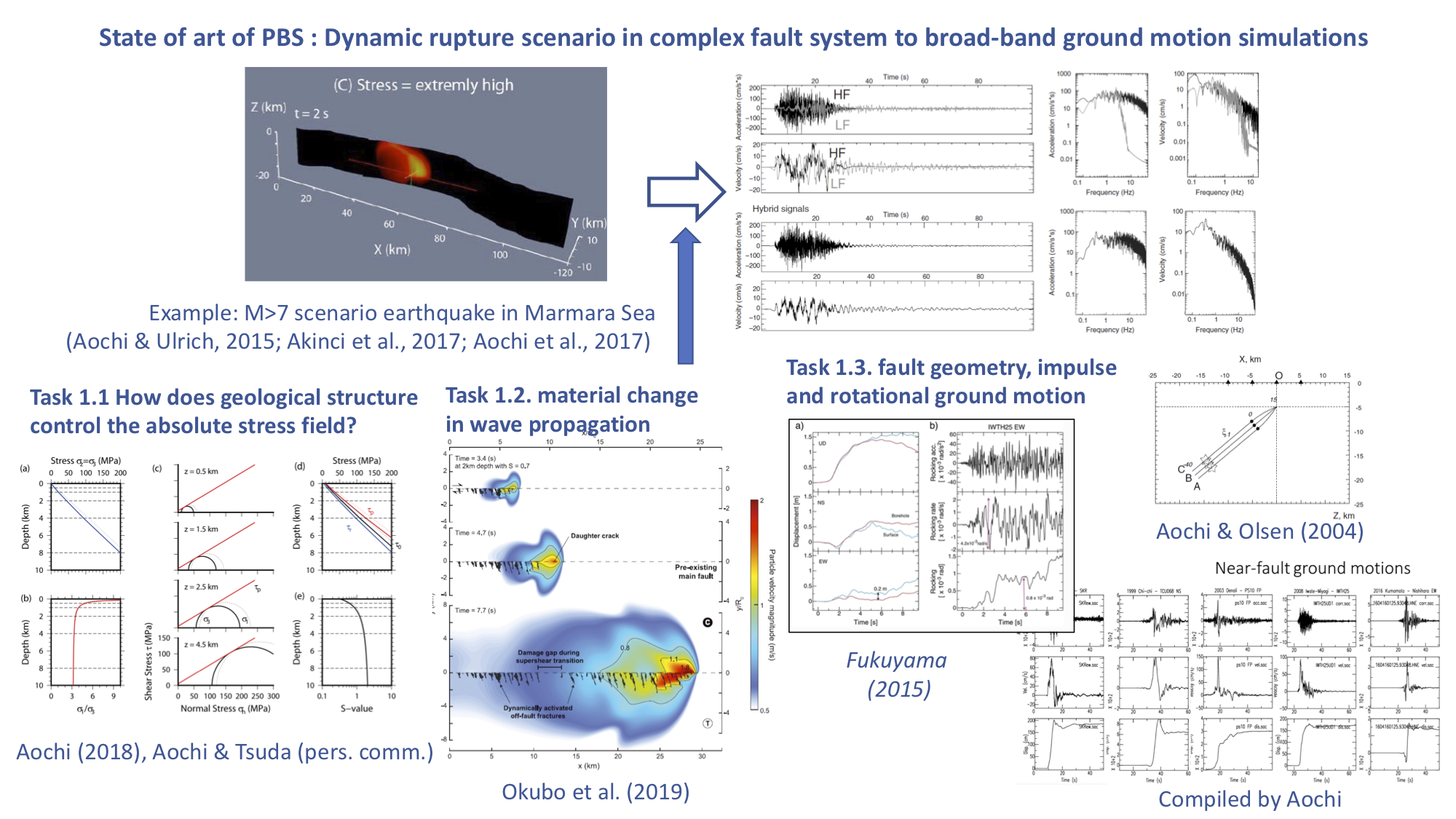
Physics-based simulations (PBSs) can be now performed by various methods, such as Boundary Integral Equation Method (BIEM), Finite Difference Method (FDM), Finite Element Method (FEM), Spectral Element Method (SEM), Discontinuous Galerkin Method (DG), and Finite Volume Method (FVM) (Harris, et al., 2018; See also the initiative of the Southern California Earthquake Center (https://strike.scec.org/cvws/code_descriptions.html). Figure 1 demonstrates an example of the state-of-art of PBS to broadband ground motion prediction coupling (1) PBS at low frequencies using BIEM-FDM and (2) stochastic simulation of high frequencies (Aochi and Ulrich, 2015; Akinci et al., 2017). Although such model allows to discuss a probable earthquake scenario and an extreme case (Aochi et al., 2017), the model setting is still oversimplified in terms of fault geometry (main fault is geometrically complex but without secondary off-plane faults), stress condition (only lateral rupture extension is focused without discussing the surface rupture probability) and medium (a simple elastic medium). The understanding of earthquake dynamics has progressed, especially thanks to the near-field seismological data and geodetic observations of the recent crustal earthquakes such as the 2016 Central Italy sequences, 2016 Kaikoura earthquake in New Zealand, 2017 Kumamoto in Japan, 2019 Ridgecrest in California, and others (Urata et al., 2017; Ulrich et al., 2019; Zhang et al., 2020). However, the near field ground motions are still difficult to understand (reproduce) without comprehending the mechanics behind, in particular, for our interest of this project, (1) initial state and boundary conditions, (2) nonlinearity in the source area (other than the site conditions) and (3) fault geometry and complex seismic wave radiation. We propose to improve these elements in PBS both from the theoretical advances and the analysis of the observational data. We keep a macroscopic vision for seismic hazard application, without always solving the microscopic mechanisms of the phenomena.

WP2 — TEMPORAL CHANGES OF MATERIAL PROPERTIES FROM EARTHQUAKE DATA

Coordination: Fabian Bonilla (UGE)

Main partners: UGE, UGA, BRGM, USC, USGS, ERI

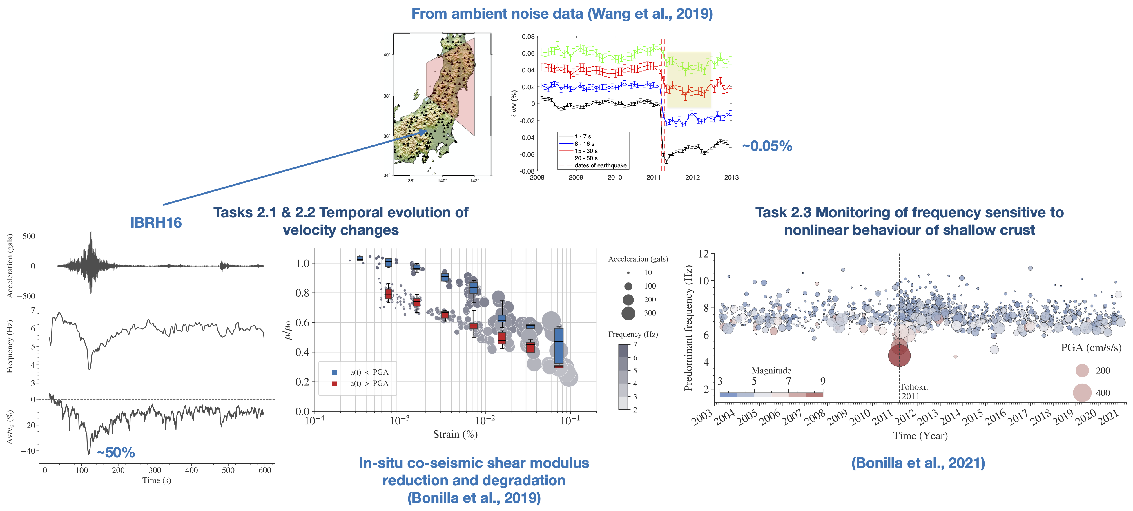
Seismic velocity changes related to earthquake activity reveal that large events induce long-term perturbations of crustal properties. For example, measured seismic velocity changes from the Mw9 Tohoku-Oki mega-earthquake that struck Japan in 2011 show velocity reduction for more than 2 years after the main event and a recovery over time (Wang et al., 2019). Similar observations and studies from other events suggest that the seismic velocity changes are related to co-seismic damage in the shallow layers and to deep co-seismic and post-seismic stress relaxation within the fault zone (e.g. Minato et al., 2012; Hobinger et al., 2016; Nimiya et al., 2017; Wang et al., 2019; Boschelli et al., 2021). In addition, the deployment of dense arrays worldwide and the development of robust signal processing methods allow measuring small velocity variations due to dynamic perturbations at the crustal scale (e.g. Brenguier et al., 2008; Wang et al., 2019). These studies generally use ambient seismic noise, which is widespread and is available in essentially all regions and time intervals (e.g. Sens-Schönfelder and Wegler 2006; Brenguier et al., 2008). However, noise sources are relatively weak, requiring stacking of relatively quiet periods, leading to time steps of days or more. Conversely, signals generated by repeating earthquakes can also been used (e.g., Poupinet et al. 1984), often involving time steps of days as well. The use of spectral ratios of seismograms recorded by different stations (e.g. Wu and Peng, 2012; Nakata and Snieder, 2012), cross-correlations of earthquake waveforms (Roux and Ben-Zion, 2014), and auto-correlation in moving time windows of seismograms (Bonilla et al. 2019; Qin et al. 2020; Bonilla et al., 2021) can achieve time resolution of minutes to seconds and resolve finer details of temporal changes, in particular co-seismic ones. Figure 2 (top) illustrates the velocity changes produced by the M9 Tohoku-Oki earthquake in 2011. The use of continuous ambient seismic noise shows up to 0.05% velocity changes in the frequency band of 0.14 to 1 Hz (1 to 7 s period), and they last for several years (Wang et al., 2019). Bonilla et al. (2019) used earthquake data from the same event recorded at station IBRH16 (KiK-net) and they found co-seismic velocity changes around 50% in the first 15 m depth (Figure 2, bottom left). This is 2 orders of magnitude higher. There is a faster recovery, compared to the whole crust, of material properties after the PGA but not completely. Velocity changes can be transformed into normalized shear modulus (Figure 2, bottom middle). The shear modulus reduction is different before and after the PGA. There is a different behavior during the loading phase (before PGA) and recovery phase (after PGA), suggesting material degradation and healing. Furthermore, this is observed at a frequency band of engineering interest (1 to 10 Hz). Figure 2 (bottom right) illustrates the time evolution of the predominant frequency for 17 years of earthquake data recorded at station IBRH16 (Bonilla et al., 2021). Tracking this frequency in sediments prone to nonlinear effects near urban areas is important to identify the vulnerability of buildings located at such sites. These are in-situ observations, and the 3 components of the ground motion can be used, and constitute an important advance to characterize in-situ nonlinear top crust’s rheology during strong ground shaking.

We will use these recently developed methods to study the nonlinear processes around the fault zone and shallow crust, to reveal the related velocity changes and the instantaneous frequency evolution during strong motion.

WP3 — CHARACTERIZATION OF THE URBAN GROUND MOTION FOR SEISMIC RISK ANALYSIS

Coordination: Philippe Guéguen (ISTerre)

Main partners: UGA, UGE, BRGM, Los Alamos, Munich University

Several recent observations prompted the initiation of the E-City project. Guéguen and Colombi (2016) reported different earthquake response of three clustered towers located in the highly amplified sedimentary basin of the Grenoble valley (France). The oscillation of the central tower was attenuated, as the other two towers acted as seismic barriers. Another observation was the confirmation, at the geophysical scale, of the concept of resonant meta-material formally defined in physics (Colombi et al., 2016). The properties of locally resonant meta-materials (in our case, buildings being the urban meta-material) are governed by interferences between incident and scattered waves, which can lead to hybrid wavefields (Lemoult et al., 2013); a similar process expected in site-city interaction. Meta-material physics have also pointed the generation of forbidden frequency bands, a phenomenon known as invisibility cloak. They are independent of the spatial ordering of the resonators when organized at the sub-wavelength scale (Kaina et al., 2013). recently, a dense array experiment using 1000 geophones deployed in the open field and in a dense forest, showed the cloaking phenomenon (Roux et al., 2018; Lott et al., 2020) and confirmed the spatial and frequency variability that a dense resonator array (a city) may have on ground motion.

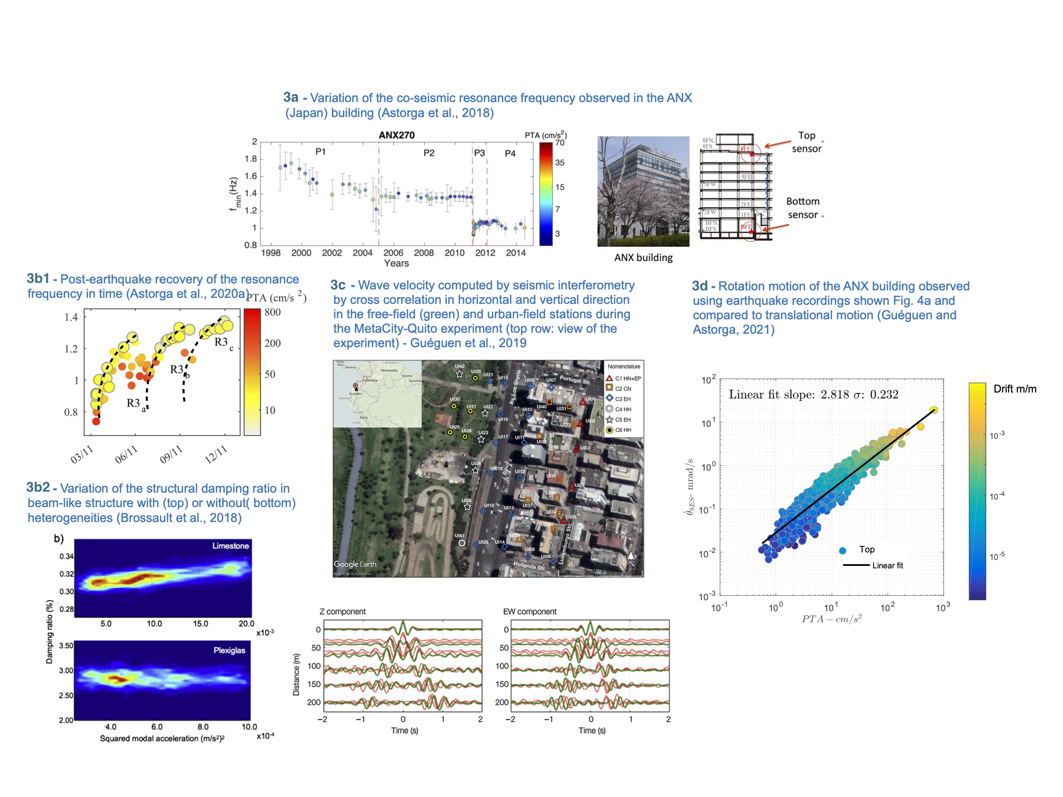
At first order, the seismic behavior of structures is controlled by their resonant frequency and damping ratio. Under strong ground shaking, the co-seismic variation of resonance frequencies is linked to possible structural damage, a key issue to estimate the vulnerability of structures (Fig. 3a). Astorga and Guéguen (2020a) analyzed the frequency shift and its recovery (Fig 3b1), showing that the latter (e.g., the slope) is a proxy of the amount of heterogeneities (or damage). Furthermore, Brossault et al (2018) observed that under ambient vibration (moderately modulated in amplitude), there is a relation between the damping variation of the structure and the number of heterogeneities (Figure 3b2). This suggests that under strong loading, the recovery of damping could be a proxy for structural damage characterization and the related nonlinear structural behavior. Tracking the variation of damping under fast-dynamic loading (in addition to the resonant frequency) is an essential challenge to understanding the seismic vulnerability of structures, especially in the near-fault condition (WP1). In addition, the seismic wavefield diffracted back into the ground by the structures contributes to the spatial variability of the seismic motion, in particular in frequency and amplitude (Fig. 3c). One may wonder what effect the linear/nonlinear transition may have on the locally resonant meta-material that constitutes the urban area. In addition, it is known that rotational motion (missed in previous studies) can be generated by the backscattered wavefield from the vibrating structures (Trifunac, 2009) and that the rotational motion in structures is important (Fig. 3d). Rotation-to-translation elastic frequency ratio Ω is a key criterion for the prevalence of ground motion rotational effects in the response of structures (Astorga and Guéguen, 2020b; Guéguen and Astorga, 2021). This raises the question of the effect of the rotation of structures on the rotation of the urban meta-material induced wavefield, which in turn contaminates the variability of the urban seismic motion. We aim to analyze the contamination of the ground motion due to the presence of clusters of urban structures, considering rotational component and spatial variability and the co-seismic nonlinear response of the structures.

WP4 — DYNAMIC RUPTURE SCENARIOS FOR THE QUITO FAULT AND BUILDING RESPONSE

Coordination: H. Aochi (BRGM), Ph. Guéguen (ISTerre), and F. Bonilla (UGE)

Main partners: BRGM, UGA, UGE, EPN, USC, USGS, ERI

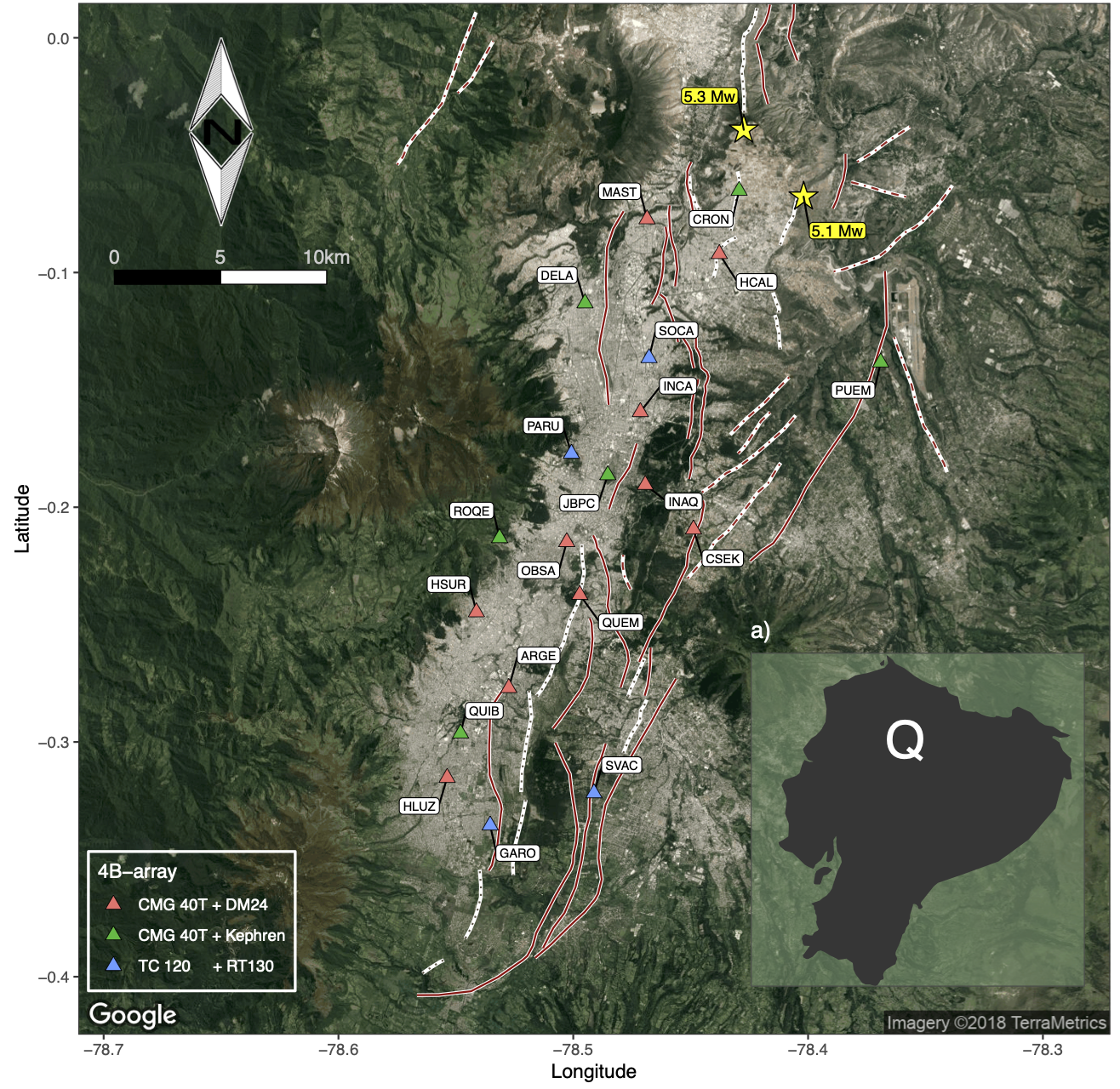
Quito Valley (population of 2.5 million inhabitants, 40km length x 5 km width, Fig. 4) is situated in a piggy-back basin developed on the hanging wall of an active reverse fault system named the Quito Fault System (QFS). In recent studies, Alvarado et al. (2014) and Mariniere et al. (2020) reported that the QFS accommodates an average of 3 - 5 mm/yr of horizontal shortening. Based on the analysis and modeling of GPS data in InSAR, a weak rate of elastic deformation accumulation and a shallow locking depth (less than 3 km) have been identified. Moreover, an aseismic slip is taking place at shallow depths in the central segment of the QFS and its associated shallow creep decreases from the center towards the south and north segments of the fault system, suggesting a heterogeneous strain accumulation in the fault system (Mariniere et al., 2020). Beauval et al. (2010) suggest that a crustal event in 1587 is probably related to the QFS with an estimated magnitude between 6.3 and 6.5. Since the development of the Ecuadorian seismological network in the early 1990s, seven earthquakes of magnitude larger than 4.0 have been recorded and located in the Quito area (Alvarado et al., 2018). Two of them had magnitudes greater than 5.0, one in 1990 (Mw 5.3) and the other in 2014 (Mw 5.1) (Figure 4), both associated to the QFS (Beauval et al., 2014).

Between 2016 and 2018, around 40 broadband stations were installed in Quito to study the basin structure using seismic interferometry (Pacheco et al, 2021). They found that the center and northern areas, the estimated basin depth and mean shear-wave velocity are about 300 m and 1700 m/s, respectively, showing resonance frequency values between 0.6 and 0.7 Hz. On the contrary, the basement’s depth and shear-wave velocity in the southern part are about 1000 m and 2600 m/s, having a lower resonance frequency value of around 0.3 Hz. In August 2018, 42 short period and broadband stations were installed in an area of 200 x 150 m2, with an interstation distance of 50 m, approximately (MetaCity Quito array, Guéguen et al., 2019). These stations were deployed both in buildings and free field, to specifically analyze the coupling between soil and structures at short wavelengths (Figure 3c). A recent study showed the period distribution and its variation during earthquake activity at several buildings in Quito (Perrault et al., 2020). Why Quito? These studies permit proposing for the first time seismic scenarios of the dynamic rupture of the Quito fault system, taking into account propagation within a sedimentary basin, and the effect of resulting ground motion on the buildings in the city. This work package joins all groups to prepare the different input models (fault, basin, and buildings), creating a natural synergy to understand the seismic risk of this city. This is a single task work package, which will become active at the beginning of the third year after we have the first outcome from WP1 to WP3. Finally, we plan to present the results of this exercise to the city of Quito, in the middle of the fourth year, in a series of scientific seminars to the authorities and public there.